Anomaly detection is a complicated and well-researched area of computer science. With all of the machine learning hype of recent months, I wanted to build something using my favorite programming language, Elixir.

In 2016, a paper called Robust Random Cut Forest Algorithm was published.
The Random Cut Forest Algorithm is an unsupervised anomaly detection algorithm that is typically used in Amazon Sagemaker (docs). It aims to improve upon the Isolation Forest Algorithm. I could have tried my hand at isolation forests, but they’re so 2008.
What makes the random cut forest algorithm different is that it measures the collusive displacement rather than just the depth of a leaf node. This measure represents how many leaves in the tree would be displaced as a result of its insertion or removal. In datasets with irrelevant features, this produces much better results.
In both algorithms, an ensemble of trees (a forest) is constructed. Each tree provides a value for a given point and they are combined to produce the result.
The solution in the LiveBook document above is written entirely in Elixir, allowing it to be invoked without NIFs. A production-grade solution might involve calling a native implementation, but it’s likely that a more efficient version could still be built in Elixir.
How RCF Works
Making a tree
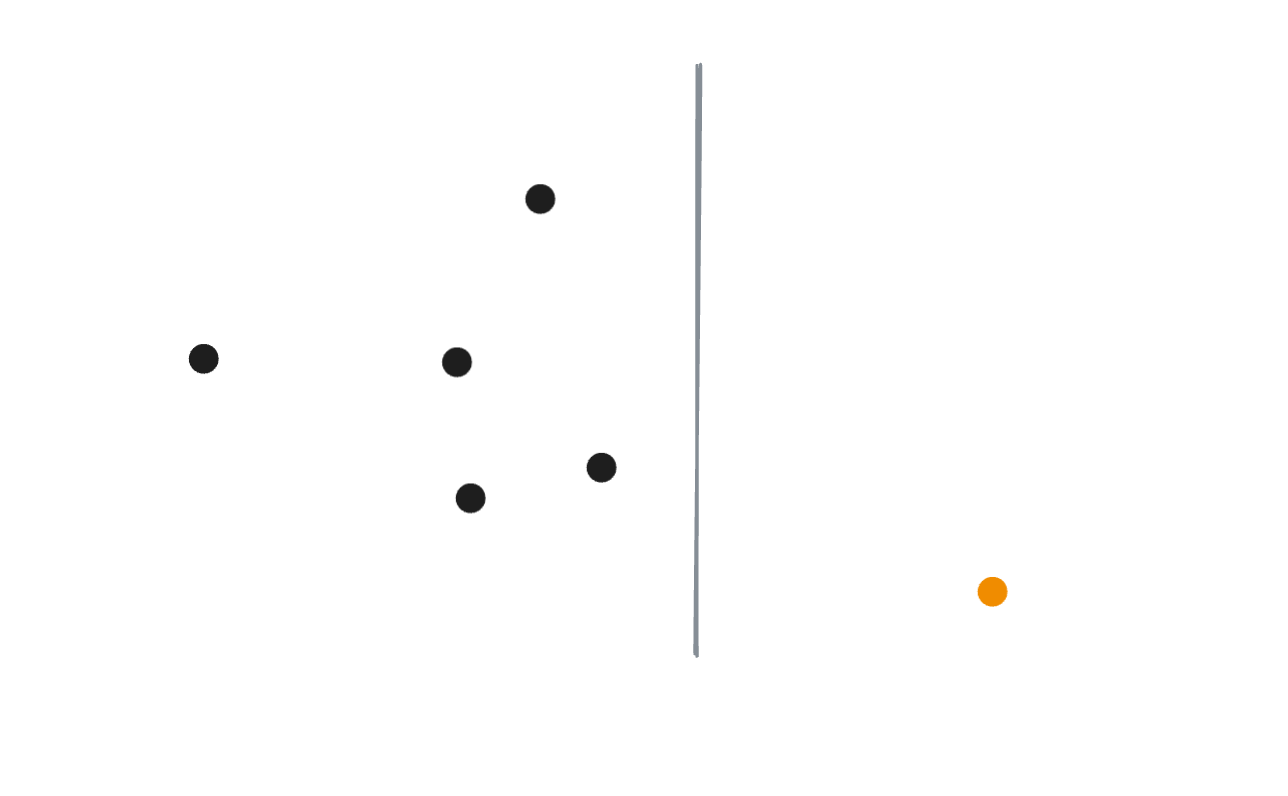
A set of multi-dimensional points are introduced to the tree. For simplicity, they will be depicted in two dimensions. In reality, any number of dimensions will do.

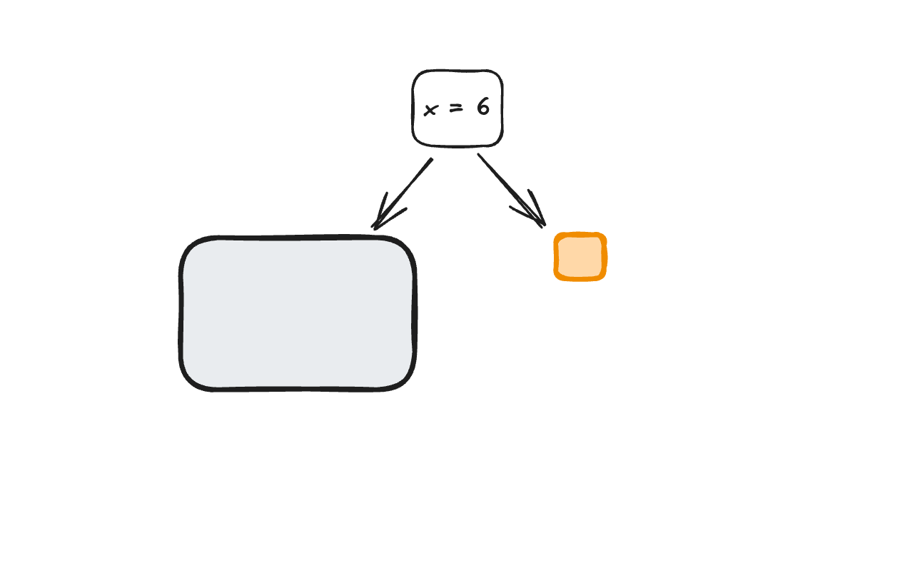
A random cut is made along a random axis, weighted by the span of each dimension’s bounding box. In this case, we randomly choose to make a vertical cut, isolating one point.

This can also be represented visually as a decision tree.

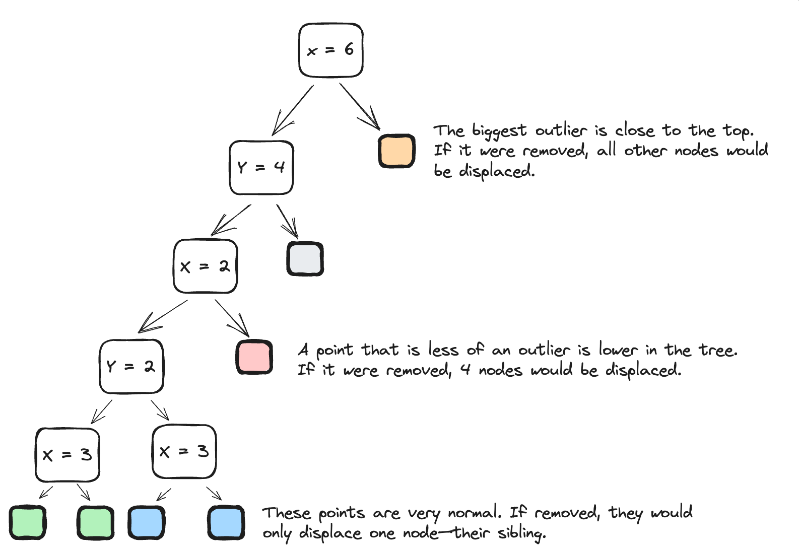
We then repeat this process until each point (leaf node) is isolated.


The Forest

A random cut forest is an ensemble of trees. Each tree is unique and learns something different about the dataset by the points it’s fed and the cuts it chooses.
Evaluation
To determine how much of anomaly a datapoint is, we insert it into the tree and calculate a collusive displacement score. This score is calculated across all trees in the forest, and the arithmetic mean is used as the result.
For example, if we were looking for the orange dot in the tree above, its score from the tree would be 6—the number of nodes that would be displaced if we were to remove it. They would be displaced because the root node would be replaced, and all branches below would be shifted up.
The displacement score of the red dot in this tree would be 4—the number of leaf nodes under its sibling. Visually, this makes sense. It’s closer to the cluster than the orange point.
Another tree might have made a different observation, deciding to cut out the red dot before the black one. This would result in a higher score.
For this reason, it’s important to consider the perspectives of the full forest.
Sine Wave Anomaly Exercise
In the research paper, the team constructs a sine wave and inserts an anomalous flat section in the middle. They then train a forest on the normal section and present the calculated anomaly scores for each point.
The linked LiveBook does the same, with some fuzziness applied to the wave for added realism.

Shingling the Data
Shingling is used to turn the time series into something periodic. Adjacent values are inserted in the tree together as multiple dimensions of the same datapoint.
For example, given a series [1, 2, 3, 4, 5] and a shingle factor of 3, the tree would receive the following multi-dimensional data points:
[1, 2, 3]
[2, 3, 4]
[3, 4, 5]
Shingling is used to represent patterns within the larger dataset. A peak is typically surrounded by lower values, and downward values typically only increase after a valley.
Final Results
With 1,000 data points, an anomaly lasting 20 steps, 50 trees containing 256 4-shingled points each, the following result is achieved:

The outlier score spikes at the beginning and end of the anomaly. There are also some smaller spikes as a result of the noise applied to the wave.

A histogram of the outlier scores shows that most scores hover around the 4–4.5 region, while a very small number of scores exceed 20—let alone 30. This analysis can be helpful in tuning the parameters of the forest as well as determining an alerting threshold.
Summary
The linked LiveBook explores a partial implementation of the approach described in the RCF paper. Along with some visuals, it has helped me build an intuition for how some random choices and a few trees can result in unsupervised anomaly detection.
If you haven’t already, try out the LiveBook locally and check out the implementation details that didn’t fit in this post:
Citations
S. Guha, N. Mishra, G. Roy, & O. Schrijvers, Robust random cut forest based anomaly detection on streams, in Proceedings of the 33rd International conference on machine learning, New York, NY, 2016 (pp. 2712-2721).
F. T. Liu, K. M. Ting and Z. -H. Zhou, “Isolation Forest,” 2008 Eighth IEEE International Conference on Data Mining, Pisa, Italy, 2008, pp. 413-422, doi: 10.1109/ICDM.2008.17.